Sharpe, Sortino and Information ratio
On this page
The Sharpe ratio is the most common way to judge a fund or a trading strategy. The Information ratio is how a manager hired to beat an index gets judged, and the Sortino ratio answers a fair complaint about Sharpe. This post covers all three.
All three build directly on mean and standard deviation.
Why you need a ratio at all
Fund A returned 12% last year, fund B 8%. Is A better? Not necessarily. If A swung wildly to get there and B was calm, B may have given you more return per unit of risk. Every ratio here has the same shape:
the ratioreturnsrisk
They differ only in what “extra” and “risk” mean.
Sharpe ratio
Plain meaning: how much return you got above a risk-free investment, for each unit of total volatility. This is the form in Romero and Balch’s What Hedge Funds Really Do (chapter 2):
| Symbol | Meaning |
|---|---|
| the portfolio’s return over the period | |
| the risk-free return over the same period (for example a short-term government bill) | |
| the excess return: what you earned for taking risk | |
| the portfolio’s standard deviation (its volatility) |
The book’s own example: the S&P 500 at 10% a year, bills at 2.5%, volatility 15% gives .
With daily data, you annualise by multiplying by :
where are the daily returns. (When the risk-free rate is the same every day, the standard deviation of and of are identical, so you’ll see both versions.)
Why and not 252? The top of the fraction (a mean) grows with time, so ×252. The bottom (a standard deviation) grows with the square root of time, so ×√252. Divide one by the other and you’re left with . (The square-root rule is explained in the standard deviation post.) For monthly data, use . For weekly, .
Worked example
Five daily returns: 1%, −2%, 1%, 2%, −1%. Risk-free rate 0, to keep it simple. From the last post, the mean is 0.2% and the standard deviation is 1.6432%.
As a rough guide, an annual Sharpe above 1 is considered good for a strategy, and above 2 is rare. Five days is far too short to trust any of these numbers, of course; this is only to show the arithmetic.
The risk-free rate per day
If the risk-free rate is 4% a year, the daily rate is the 252nd root of the yearly growth:
The shortcut is close enough for most uses. Many people simply use 0 when rates are very low.
What Sharpe gets wrong
The standard deviation punishes all swings, up and down. A fund with a few huge gains gets penalised exactly like a fund with a few huge losses. Investors don’t mind upside surprises.
Sortino ratio
Plain meaning: like Sharpe, but only the bad days count as risk.
| Symbol | Meaning |
|---|---|
| the target return, often 0 or the risk-free rate | |
| how far a day fell short of the target; 0 on days that beat it | |
| DD | downside deviation: the typical size of a shortfall |
Good days count as zero shortfall, so they don’t add to the risk. Note that the average is over all days, good and bad. That’s the common convention; some references divide by the number of bad days only, which gives a different number, so always check which one a report uses. Annualise with , as before.
Worked example
Same five days, target 0:
| Day | Return | Squared | |
|---|---|---|---|
| 1 | 1 | 0 | 0 |
| 2 | −2 | −2 | 4 |
| 3 | 1 | 0 | 0 |
| 4 | 2 | 0 | 0 |
| 5 | −1 | −1 | 1 |
| Average | 0.2 | 1.0 |
Higher than the Sharpe of 1.93, because the up days no longer count against the fund.
Where Sortino earns its keep
I made up three funds with exactly the same mean and standard deviation, so their Sharpe ratios are identical. Only the shape differs:
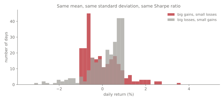
| Fund | Sharpe | Sortino | Worst day | Best day |
|---|---|---|---|---|
| Symmetric | 0.705 | 1.025 | −3.05% | +2.57% |
| Big gains, small losses | 0.705 | −1.01% | +6.21% | |
| Big losses, small gains | 0.705 | −6.53% | +0.99% |
(Risk-free rate 4% a year.) Sharpe can’t tell them apart. Sortino ranks the “big losses” fund clearly worst, which is what an investor would say too. Strategies that sell insurance-like options often look like that last fund: steady small gains, then a rare large loss. Their Sharpe can look excellent right up until the bad day.
Information ratio
Plain meaning: how much a manager beat their benchmark, for each unit of straying from it.
A fund manager is usually hired to beat an index, not cash. So “extra return” becomes the return above the index (the active return), and “risk” becomes how much the fund’s return differs from the index’s (the tracking error). This is the version in Grinold and Kahn’s Active Portfolio Management:
where is the fund’s return and the benchmark’s.
Romero and Balch (chapter 9) measure skill the same way, but on alpha: the part of the return left after removing what the market explains, using the CAPM (the capital asset pricing model):
For a fund that moves one-for-one with its index (a beta of 1), alpha is simply fund minus index, and the two versions agree.
Worked example
Same five fund days, plus a benchmark: 0.5%, −1.5%, 1%, 1.5%, −1%.
| Day | Fund | Benchmark | Active |
|---|---|---|---|
| 1 | 1 | 0.5 | 0.5 |
| 2 | −2 | −1.5 | −0.5 |
| 3 | 1 | 1.0 | 0 |
| 4 | 2 | 1.5 | 0.5 |
| 5 | −1 | −1.0 | 0 |
Active returns: mean 0.1%, standard deviation 0.4183%.
Two managers
| Manager | Beats index by | Tracking error | IR |
|---|---|---|---|
| A: stays close to the index | 1% a year | 2% a year | |
| B: takes big bets | 3% a year | 12% a year |
B earned three times more extra return, but took six times more risk relative to the index. Per unit of risk, A is twice as good. If you like A’s skill but want more return, you can give A more money to work with, or let A take bigger positions. B’s extra return came with a lot of noise.
The IR leads to the Fundamental Law of Active Portfolio Management, from Grinold and Kahn, as Romero and Balch write it in chapter 9:
In plain words: a manager’s IR comes from how good each bet is (the information coefficient, IC, the correlation between forecasts and what actually happened) times the square root of how many independent bets they make each year (the breadth, BR). Small skill applied many times can beat big skill applied rarely. That’s a post of its own.
The code
import numpy as np
K = np.sqrt(252)

def sharpe(r, rf=0.0):
    ex = r - rf
    return K * ex.mean() / ex.std(ddof=1)

def sortino(r, target=0.0):
    downside = np.sqrt(np.mean(np.minimum(r - target, 0) ** 2))
    return K * (r - target).mean() / downside

def info_ratio(r, benchmark):
    active = r - benchmark
    return K * active.mean() / active.std(ddof=1)

r = np.array([1, -2, 1, 2, -1]) / 100
b = np.array([0.5, -1.5, 1, 1.5, -1]) / 100
print(sharpe(r), sortino(r), info_ratio(r, b))    # 1.93  3.17  3.79
Summary
| Ratio | Extra return | Risk | Use it when |
|---|---|---|---|
| Sharpe | above risk-free | all volatility | comparing any two investments |
| Sortino | above a target | only shortfalls below the target | returns are lopsided (options, credit) |
| Information | above a benchmark | tracking error | judging a manager hired to beat an index |
All three: annualise daily figures with , and never trust them on a short history.
Next
Portfolio optimisation: using means, standard deviations and correlations together to find the mix of assets with the best risk-adjusted return.
References
- Philip J. Romero and Tucker Balch, What Hedge Funds Really Do: An Introduction to Portfolio Management (Business Expert Press, 2014), chapter 2 (the Sharpe ratio) and chapter 9 (the information ratio on alpha, and the Fundamental Law IR = IC × √BR)
- Richard C. Grinold and Ronald N. Kahn, Active Portfolio Management (2nd ed., McGraw-Hill, 2000)
- William F. Sharpe, “The Sharpe Ratio”, The Journal of Portfolio Management 21(1), 1994
- Frank A. Sortino and Lee N. Price, “Performance Measurement in a Downside Risk Framework”, The Journal of Investing 3(3), 1994 (the Sortino ratio is not in the books above)